Snowflake Query Profile: An Autopsy for Slow Queries

If you think a slow query’s SQL text will tell you why it was slow, think again. All you’ll see is what the user asked for, not what actually happened. Indeed, two queries with identical text can have wildly different executions due to differences in the data and environment. This includes how many partitions got read, whether the join multiplied rows, or whether the working set fit in memory.
Donald Knuth said the quiet part out loud back in 1974: premature optimization is the root of all evil. Still, we shouldn’t pass up our opportunities in the small number of places where performance truly matters: what Knuth calls the “critical three percent.”
So how do you find that critical three percent? And how do you validate that it’s truly “critical”? Like anything, you measure. And with Snowflake, the measuring instrument at your disposal is the Query Profile. Snowflake builds one for every query it executes; but almost nobody opens them.
In this article, we’ll walk through what the Snowflake Query Profile is, how to use it, and, perhaps most importantly, what it won’t tell you.
Key Takeaways
- The Snowflake Query Profile shows you how a given query actually ran, not what your SQL asked for. It maps every operator and the row counts flowing between them.
- Users should read Snowflake Query Profile in a fixed order. We recommend the most expensive nodes first, then execution-time clock, spill, pruning, and row counts. That sequence turns a slow query into a specific mechanism.
- The profile is retrospective and allows visibility into one query at a time. It flags an inefficient query but won’t tell you which fix is worth your time. While helpful for one-offs, it’s not a scalable solution.
Table of Contents
What is the Snowflake Query Profile?
The Snowflake Query Profile is a visual representation of how specific queries are executed inside the platform. Snowflake details the individual processing steps of each query and compiles them in a comprehensive performance and resource breakdown. This includes the following:
| Query Metadata | Query ID, Session ID, and Query Tag. |
| Query Execution Plan | A visual graph showing the sequence and structure of operations (or nodes) that were performed during the query’s execution. |
| Execution Statistics | These are the metrics illustrating the nature and scope of each operation, including the number of rows processed, data scanned, and execution time (both for each step and for the overall query). This information also shows how many micro-partitions were scanned out of the total available. |
| Resource Usage | This gives you insights into CPU processing, disk I/O, synchronization and initialization, network transfer, and more. |
| Error and Warning Messages | Any errors or warnings encountered during query execution. |
| SQL Text | The SQL statement that was executed. |
Execution Plan: Operators and Links
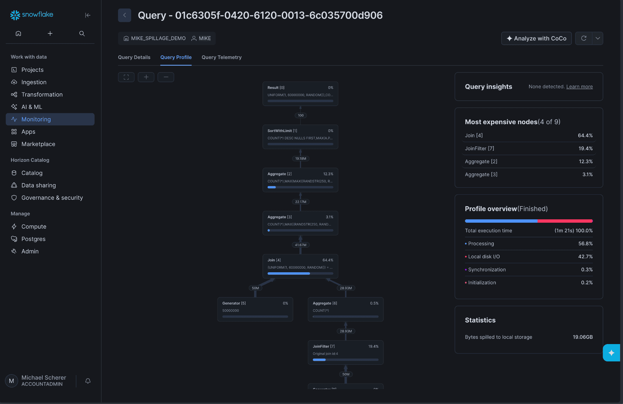
The part of the Snowflake Query Profile that takes more practice to read is the execution plan itself. What we listed above is easy by comparison. So it’s worth knowing what exactly it contains before you open one.
First, a quick clarification: when you submit SQL, Snowflake’s optimizer does not run your text. It compiles that text into a plan: the sequence of steps it judges to be the cheapest way to produce your answer. Because the optimizer decides the order, the plan can look nothing like the order you wrote your query in. That is the optimizer doing its job, not a defect to correct.
The execution plan is a graph consisting of two things:
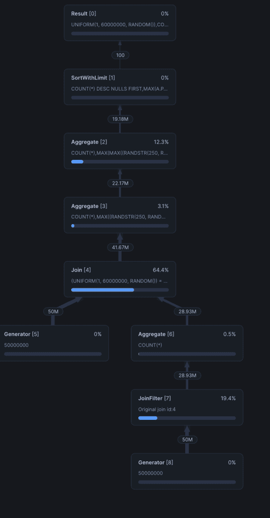
- Operators (or nodes). These are the units of work: read a table, filter rows, join two inputs, aggregate, sort, return the result. Each node shows a type that tells you what it did and a percentage that tells you how much of the query’s total time it cost.
- Links. These are the arrows between operators, indicating the count of rows passing from one node to the next.
Keep in mind that execution flows from bottom to top. Which means the lowest nodes in each branch are almost always TableScans pulling data off storage, while the single node at the top is usually a Result.
If you read the graph upward, the row counts along the links will show you where rows were created that never should have existed in the first place.
A Field Guide to the Operators You’ll Meet
Snowflake emits a lot of operators; there’s no need to memorize them all. You just need to know the dozen or so that turn up in real queries. More importantly, you should be able to tell at a glance which are innocuous, and which ones cause queries to run slow.
| Operator | What It Does | What to Watch For |
|---|---|---|
| TableScan | Reads columns from a table, off remote storage or local cache. | Usually your most expensive node, which is normal. Judge it by pruning: partitions scanned against partitions total. |
| Filter | Applies your WHERE conditions. | Rows in often equals rows out, because Snowflake pushes filters down into the TableScan. Not a sign the filter did nothing. |
| Join | Combines two inputs on a key. | The single richest source of trouble. Output rows exceeding both inputs is an exploding join. |
| JoinFilter | Derives a filter from one side of a join and applies it to the other. | Good news, not a problem. It prunes partitions with no WHERE clause of your own. |
| Aggregate | Runs GROUP BY and functions like SUM, COUNT, AVG. | An Aggregate stacked on a UnionAll is a UNION quietly deduplicating rows that were never duplicated. |
| Sort / SortWithLimit | Orders rows for ORDER BY, or applies LIMIT. | Sorts are expensive. An early sort the query never needed is money spent on nothing. |
| UnionAll | Stacks two row sets. | Harmless with ALL. With a bare UNION, an Aggregate appears on top to remove duplicates that were never there. |
| WithClause / WithReference | A CTE, computed once and referenced thereafter. | Everything downstream waits on it. One slow CTE can stall the whole branch beneath it. |
| Result | Usually the final node. Returns the answer. | Cheap, and never the problem. |
How Do I Use the Snowflake Query Profile
First, you need to find it: in Snowsight, go to Monitoring > Query History, select the query in question, and open the Query Profile tab. Profiles are available for 14 days after they complete. Queries that fail to run have no profiles.
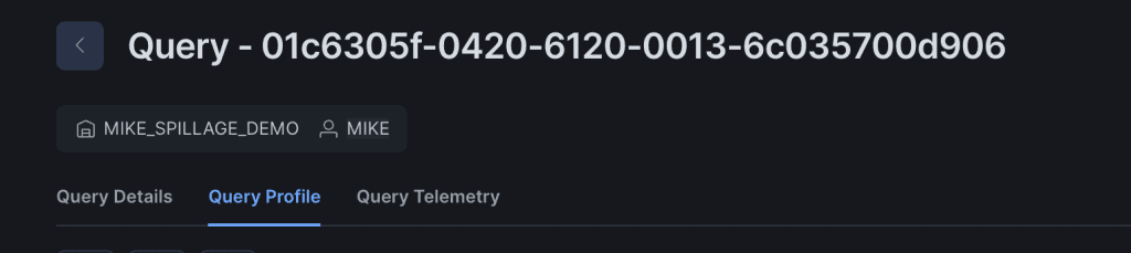
There are other, faster ways to access the Query Profile, depending on where you are in Snowflake:
- In a Worksheet, run a query and you’ll find the profile in the results pane
- In the newer Workspaces interface, hover the information symbol in the Results pane and click the query ID.
- In a Snowflake Notebook, click the duration at the top of an executed SQL cell, then the query ID.
And if you already have the query ID in hand, skip the clicking entirely. Snowflake’s console uses structured URLs, so you can jump straight to any profile by filling in a template:
https://app.snowflake.com/<region>/<account-locator>/compute/history/queries/<query-id>/profileThe profile is not only a UI. The same per-operator numbers are available in SQL through the GET_QUERY_OPERATOR_STATS table function, which you wrap in TABLE() and point at a query ID.
Two constraints are worth knowing before you execute this command:
- It returns rows only for queries that have already completed.
- You need OPERATE or MONITOR on the warehouse that ran them.
- It is capped at 14 days
The best move is to pair it with the QUERY_HISTORY account usage view, which retains roughly a year of history. Rank the account’s worst queries there—by execution time, by bytes spilled—and then pull operator stats only for the handful that deserve an autopsy.
That two-step pattern is what turns profile reading from a slow, stagnant process into a scalable solution.
Step 1: Ignore the Diagram & Read the Most Expensive Nodes
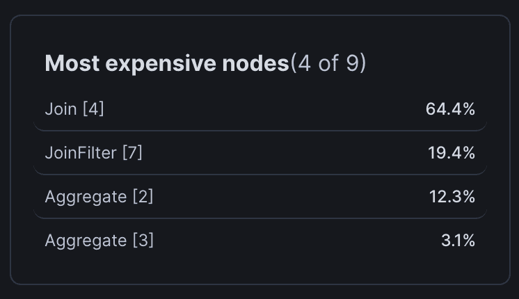
The execution plan diagram is the most eye-catching thing on the screen and the last thing you should study. Start with the Most Expensive Nodes pane, which lists every operator that consumed one percent or more of execution time, sorted descending.
Most slow queries are not uniformly slow. They have one or two operators eating the clock, and this pane names them immediately. For example:
- A TableScan at 85 percent is a scanning problem.
- A Join at 70 percent is a join problem.
- A Sort at 60 percent is a memory problem waiting to be confirmed.
Once you know which node to interrogate, you can drill down to find the actual issue.
Step 2: Read the Clock
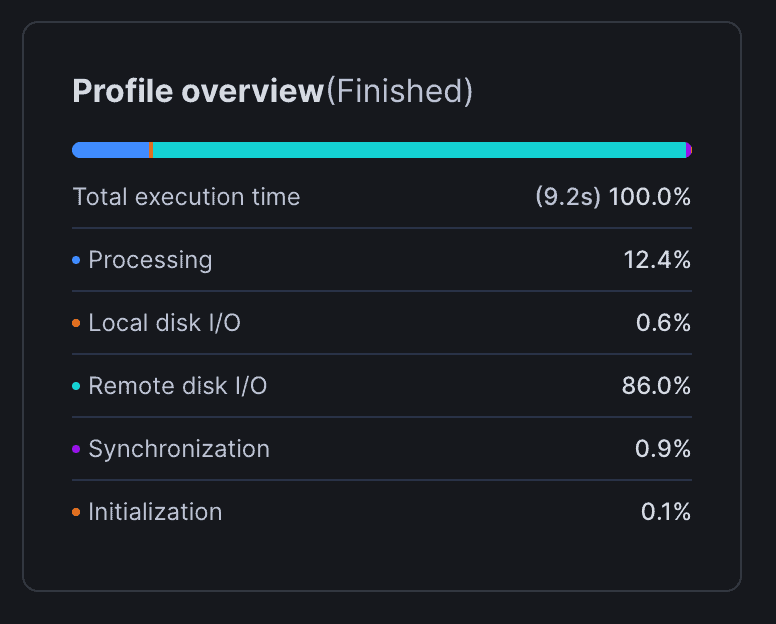
The Profile Overview pane splits execution time into categories:
- Processing dominant means the CPU was actually computing; the query may simply be big.
- Local Disk IO dominant means the working set did not fit in memory and the query paid a disk penalty.
- Remote Disk IO dominant is the alarm bell: the query was blocked on cloud storage, which usually means either a huge scan or spilling past local disk, and either way the warehouse spent your credits waiting on the network.
- High Synchronization is the subtle one, and often the fingerprint of skew: parallel workers standing around waiting for one overloaded colleague to finish.
Step 3: Check the Spill Gauge
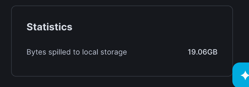
In the Statistics pane, the Spilling section shows bytes spilled to local storage and bytes spilled to remote storage. These two numbers confirm or acquit the memory hypothesis from step two.
Nonzero local spill means the operator outgrew memory. Nonzero remote spill means it outgrew local disk too, and the performance penalty is severe.
Snowflake’s own guidance offers two remedies: a larger warehouse or smaller batches of data. Which one is cheaper is an empirical question about your workload, but the profile has done its job: the slowness now has a mechanism instead of a mood.
Step 4: Check the Pruning Ratio
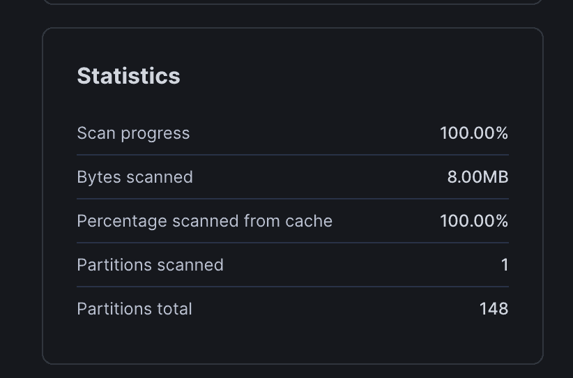
Same pane, but this time we look at the Pruning section. Partitions scanned against Partitions total. Snowflake keeps statistics on every micro-partition so it can skip the irrelevant ones, but pruning only works when the data’s storage order correlates with your filters.
Scanned as a small fraction of total means pruning is doing its work. Scanned approaching total on a filtered query means the engine read almost everything to return almost nothing, and no warehouse size will fix data organization.
While you are there, glance at Percentage scanned from cache: a repeated query reading heavily from cache is quietly telling you what its warehouse’s suspend settings are worth.
One happy surprise lives in this pane too. If you see a small fraction of partitions scanned on a table you never explicitly filtered, that is the JoinFilter operator at work: Snowflake derived a range from the other side of a join and used it to prune the table for you, for free. Good pruning without a WHERE clause is not a mystery. It is the optimizer operating within its parameters.
Step 5: Follow the Rows
Now, return to the diagram. Arrows between operators carry row counts, and you’re looking for an operator that emits far more than it consumes. Snowflake’s documentation names this the exploding join: a missing or too-loose join condition producing orders of magnitude more tuples than either input, usually with the Join node also topping the expense list.
Its quieter cousin is UNION without ALL, which appears in the profile as a UnionAll operator with an unexpected Aggregate stacked on top, silently deduplicating rows that were never duplicated.
Two footnotes on reading the arrows:
- A Filter node whose input and output row counts match did not fail. Snowflake most likely pushed your predicate down into the TableScan and discarded rows while reading, before the Filter ever saw them, so you judge filtering by partitions pruned below, not by the arrows around the Filter.
- The exploding join has an uglier extreme: the Cartesian join, where there is no usable condition at all and every row on one side pairs with every row on the other, output equal to the two inputs multiplied. Almost nobody types one on purpose. A stray range or inequality join is the usual door it walks in through.
Let Snowflake Read It With You
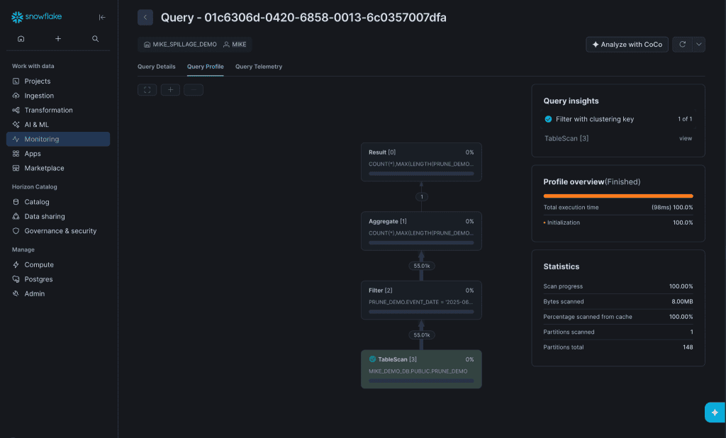
Two additions since most people last looked at this tool. The Query Insights pane now flags conditions that affected performance and suggests next steps, and the same findings are queryable in the QUERY_INSIGHTS view, which means the diagnoses above can be harvested in bulk instead of one browser tab at a time.
And the entire Snowflake Query Profile is available programmatically:
SELECT operator_id, operator_type, operator_statistics, execution_time_breakdown FROM TABLE(GET_QUERY_OPERATOR_STATS('<query_id>'));GET_QUERY_OPERATOR_STATS returns the per-operator numbers as rows, which turns profile reading from a ritual into a pipeline.
The five steps above become a script that runs against every expensive query from last week.
What Will Snowflake Query Profile Not Tell You?
Snowflake Query Profile has three limits:
- The profile is retrospective: it explains a query that already ran and already billed you.
- It enables you to review only one query at a time: nobody is going to open ten thousand profiles, and the script version still needs someone to read its output.
- It has no direct price information: you get bytes, rows, and percentages. You’ll also get an approximate credit attribution, but not an exact count of credits consumed.
That’s where Keebo comes in. The workloads my team at Keebo watches drift week over week, and the queries that deserve an autopsy this month are not the ones that deserved it last month. That is why we built the platform to continuously and autonomously monitor warehouses, with the reading of these same gauges done by machine, inside SLA guardrails you define.
Use the query profile for the deep reads. Just don’t mistake owning a microscope for having a monitoring system. The former helps you interrogate problems after the fact; the latter helps you stop the issues before they even happen.
Frequently Asked Questions
Does the Query Profile Show Query Cost?
Partly. The Query Details tab now shows an approximate credit attribution for that single execution, so you are no longer estimating from execution time and warehouse size alone. The profile prices nothing at the operator level, (you get time, bytes, rows, and partitions, not the credits each node burned) and nothing here rolls a workload up.
What Is a Cartesian Join in the Query Profile?
A Cartesian join is a join with no usable condition, so every row on one side pairs with every row on the other, and the output equals the two inputs multiplied together. It is the extreme form of an exploding join, and it almost never gets typed on purpose.
Why Do Rows In and Rows Out of My Filter Node Match?
Because Snowflake pushed your WHERE clause down into the TableScan before the Filter ever ran. This is predicate pushdown, and it is the optimizer being efficient: it discards rows while reading, so fewer of them reach the Filter above. The catch is that the profile does not show how many rows the pushed-down predicate eliminated at the scan, so a Filter that looks like it did nothing may have done its work one node earlier.
How Do I Read Query Insights in the Profile?
When Snowflake recognizes a condition worth knowing, (an exploding join, a join with no condition, a not-applicable filter) it highlights the guilty operator in yellow, marks it with a warning symbol, and explains the finding in the Query Insights pane. Treat it as a lead, not a verdict. An insight on a node that also tops your Most Expensive Nodes list is worth acting on now. An insight on a node costing two percent of the query is worth noting and moving past.
What’s the Difference Between Snowflake Query Profile and Data Profile?
They sound alike but answer completely different questions. The Query Profile explains an execution: which operators cost time, where a query spilled, and where it scanned too much. The Data Profile describes contents: row counts, null counts, min and max values, most common values, and how each column is distributed.
What’s the Difference Between Query Profile, Query Details, and Query Telemetry?
They are three tabs on the same screen, and each answers a different question. Query Details is the record of the run: status, timings, warehouse size, SQL text, approximate credits, and results. Query Profile is the execution plan: operators, timings, spill, and pruning. It is the tab that explains why a query was slow. Query Telemetry is the logs, traces, and metrics your code emitted while it ran, shown as a trace of spans.